Monetary Policy and Aggregate Demand

From FFR to aggregate demand

Lower the federal funds rate and short-term borrowing costs fall. Mortgage rates, auto loans, business loans, and consumer credit all re-price, with a lag. Lower borrowing cost raises interest-sensitive spending — residential investment, business fixed investment, durable goods purchases — shifting aggregate demand right. Higher rates do the reverse.

In AD-AS terms:

• Expansionary monetary policy (↓ FFR ⇒ ↓ market rates): AD shifts right. In the short run, real GDP rises and the price level rises.
• Contractionary monetary policy (↑ FFR): AD shifts left. Real GDP falls and the price level falls (or rises more slowly).

Preset— Custom —Baseline (calibrated)Demand boom (consumer optimism + fiscal stimulus)1973 oil shock (supply contraction)2008 demand collapse2020 pandemic (combined shock)

Default calibration. AD and SRAS cross at Y ≈ Yn, P ≈ Pe.

G

M

Expected price Pᵉ

Natural output Yₙ

Reset

Equilibrium:Y* = 1030P* = 4.00

AD ↔SRAS ↔

Pin current as snapshotCopy share link

Short-run AD-AS. AD slopes down in (Y, P); SRAS slopes up around Yₙ. Demand shocks shift AD; supply shocks change Pᵉ or Yₙ. Drag the AD or SRAS pill on the right edge, use sliders, or pick a preset.

Slide the money-supply lever in the chart and watch AD shift. Notice that the price-level response is dampened by SRAS slope — most of the shock initially shows up in output, with the price level catching up over quarters as expectations adjust.

The dynamic AD-AS model

A static snapshot misses two important things: the economy and prices both grow over time, and policy works with lags. The dynamic AD-AS model adds two features:

1. Long-run aggregate supply shifts right each period at the trend growth rate (~2% real GDP per year for the US).
2. Aggregate demand shifts right each period at a baseline driven by population, productivity, and money growth.

In the dynamic version, “contractionary” monetary policy doesn’t mean AD shifts left — it means AD shifts right by less than it normally would. Inflation falls (or stays flat) but output keeps growing, just more slowly. This is the textbook “soft landing” scenario.

How the Fed actually sets the target

In broad strokes the Fed leans against whatever is out of balance:

• Inflation above 2%? Raise rates. The further above, the more aggressively.
• Output below potential / unemployment above the natural rate? Lower rates.
• Both at once (stagflation)? You’re in the Volcker-1980 / Powell-2022 bind — fighting inflation usually wins, with output paying the cost.

There’s a formula called the Taylor rule that captures this pattern with about four numbers (current inflation, the target inflation, the output gap, and an equilibrium real rate). You don’t need to memorize it — the test is whether you can predict the direction the Fed will move when you read the next inflation print or unemployment report. If you can, you’re using the model correctly.

Crisis-era policy: 2008 and 2020

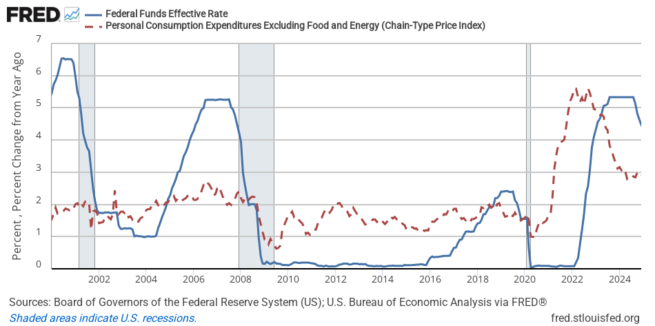
2007-2009 financial crisis. The Fed cut the FFR from 5.25% to 0-0.25% by December 2008, hitting the zero lower bound (ZLB). With the conventional tool exhausted, the Fed turned to:

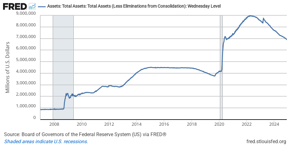
• Quantitative easing (QE) — large-scale purchases of Treasuries and MBS to push down long-term yields, expanding the balance sheet from ~$900B to over $4T by 2014.
• Forward guidance — promises about future policy (“rates will remain low for an extended period”) to reshape rate expectations.
• Special lending facilities — TAF, PDCF, AMLF, TALF — to backstop specific market segments.

2020 pandemic recession. The Fed cut from 1.75% to 0-0.25% in two weeks (March 2020), restarted QE at unprecedented pace, and stood up 13(3) emergency facilities to support corporate credit, money-market funds, and Main Street lending. The balance sheet roughly doubled, reaching ~$9T by 2022.

The 2022-2026 tightening. As inflation ran above target through 2021-2022, the Fed lifted the FFR from 0-0.25% to 5.25-5.50% by mid-2023, the fastest tightening cycle since Volcker. Quantitative tightening (letting securities mature without reinvestment) shrank the balance sheet by ~$2T. Inflation cooled materially without a sharp recession — the “soft landing” that earlier crisis-era easing made plausible.

What’s hard about all of this

Three things make monetary policy genuinely difficult:

1. Lags. Peak output effects come 12-18 months after a rate change; peak inflation effects, 18-24 months. Policy works on the economy of tomorrow, not today.
2. Unobserved variables. $r^*$, $y^*$, and $\pi^T$ are all estimated, not measured. Real-time estimates revise.
3. Expectations. Inflation today depends partly on inflation expected tomorrow. Anchoring expectations is half the job; once they unanchor (as in the 1970s) it takes a recession to re-anchor.