The IS-LM Model: Output and Interest Together

Looking for a step-by-step version? This same material is also available as a guided walkthrough that breaks it into 5 bite-size steps with a check after each.

The story IS-LM is trying to tell

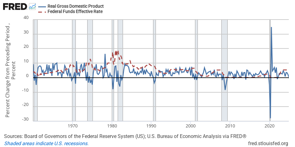
Consider what happened in late 2022. Inflation was running near 9%. The Fed had raised the federal-funds rate from near zero to about 4.5% in nine months. Mortgage rates jumped from 3% to over 7%. Homebuilders like Lennar started offering buyers thousands of dollars in mortgage- rate buydowns just to keep deals closing. New-home sales fell sharply.

Two questions the IS-LM model is built to answer:

1. When the Fed raises rates, why does output fall (not just home sales)?
2. If Congress had simultaneously cut taxes by the same dollar amount the Fed tightened, would the two have just cancelled out?

We need two curves to answer these. One for the goods market (IS) and one for the money market (LM). Where they cross is the short-run equilibrium pair $(Y, r)$.

The IS curve: every borrower’s friend

IS = “Investment equals Saving” — equivalently, every $(Y, r)$ point where the goods market clears. The intuition: lower interest rates make it cheaper for firms to borrow and invest, so they invest more, which boosts output. Hence IS is downward-sloping in $(Y, r)$: lower $r$ → higher $Y$.

What shifts IS?

• Government spending up (Congress passes a stimulus): IS shifts right at every $r$.
• Consumer confidence up (households spend a larger share of income): IS shifts right.
• Business confidence up (firms invest more at every $r$): IS shifts right.

The mechanism in one sentence: anything that raises spending at a given interest rate pushes IS right.

The LM curve: where the money market clears

LM = “Liquidity equals Money supply” — every $(Y, r)$ point where money demand equals money supply. Higher $Y$ means more transactions, which means more demand for money. To keep the market clearing at a fixed money supply, the price of money (the interest rate) must rise. So LM is upward-sloping.

What shifts LM?

• Money supply up (Fed expands its balance sheet, lowers its policy rate target): LM shifts right at every $Y$.
• Money demand shifts (panic-driven demand for cash in a financial crisis): LM shifts left.

The mechanism in one sentence: anything that raises the supply of money relative to demand pushes LM right and the interest rate down.

Equilibrium: where they cross

The short-run economy sits at the unique $(Y^\*, r^\*)$ where IS meets LM. Both markets clear at the same instant.

Preset— Custom —Baseline (calibrated)1981 Volcker tightening2008 fiscal stimulus (ARRA)2020 pandemic response2022 Fed tightening

Default calibration. Use as your anchor before applying a shock.

Government spending G

Money supply M

Autonomous spending C₀+I₀

Reset

Equilibrium:Y* = 263.2r* = 3.16%

IS ↔LM ↔

Pin current as snapshotCopy share link

Closed-economy IS-LM. Parameters: c = 0.6, t = 0.2, b = 20, k = 0.5, h = 10, P = 1. The IS curve slopes down (lower r ⇒ more investment ⇒ higher Y). The LM curve slopes up (higher Y ⇒ more money demand ⇒ higher r to clear the money market at fixed M). They cross at equilibrium. Drag sliders, type values, drag the IS or LM label directly, or pick a historical preset.

Try the sliders. Three patterns you should be able to predict before dragging:

Shock	Curve	Y* moves	r* moves
Fiscal expansion (↑ G or tax cut)	IS right	up	up
Monetary expansion (↑ M)	LM right	up	down
Confidence boom (↑ C₀ or I₀)	IS right	up	up

Back to the 2022 puzzle

The Fed’s rate hikes in 2022-2023 were a leftward shift of LM (tightening money). Equilibrium moved up the IS curve to a higher $r$ and lower $Y$. Why output fell rather than just home sales: the IS curve doesn’t track home sales — it tracks total output, including business investment, durable-goods consumption, and other interest- sensitive components. All of them respond to higher $r$.

Would a simultaneous tax cut have cancelled the Fed out? Not exactly. A tax cut shifts IS right while tight money shifts LM left. The Y effects could roughly cancel, but $r$ would rise even more. So borrowers (homebuyers, businesses, the federal government itself) would face higher rates than under the Fed alone. The two policies do different things to the equilibrium even when they’re sized to offset each other on $Y$.

A small note about the math

The model can be written down compactly as

$$Y_{IS}(r) = \alpha (A - b r) \qquad r_{LM}(Y) = (k Y - M/P)/h,$$

with $\alpha = 1/(1 - c(1-t))$ the multiplier. We use the parameters $\alpha = 1.92$, $b = 20$, $k = 0.5$, $h = 10$ in the chart. You don’t need to memorize this. You do need to remember the curve directions and what shifts each one.