Annuities and Perpetuities

Why these formulas exist

Many real-world cash-flow streams have the same shape: a fixed payment every period, for a long time. Examples:

• A 30-year mortgage: 360 equal monthly payments.
• A pension annuity: monthly payments until death.
• A consol bond (UK, 1751-2015): fixed coupon, forever.
• A preferred share: fixed dividend, indefinitely.

Discounting each cash flow individually is tedious. For repeating streams, there’s a closed-form formula. Memorize four; everything else in fixed-income valuation builds on them.

Perpetuity: a fixed payment forever

A perpetuity pays $C$ every period starting next period, forever. Its PV:

$$PV = \frac{C}{r}.$$

Quick proof: the PV equals $C/(1+r) + C/(1+r)^2 + \ldots$. This is a geometric series with first term $C/(1+r)$ and ratio $1/(1+r)$, summing to $C/r$.

Example. A perpetuity paying $1,000 per year with $r = 5\%$ is worth $1000 / 0.05 = $20,000 today. Note the inverse relationship: at $r = 2.5\%$, the same perpetuity is worth $40,000. Long-duration streams are very sensitive to the discount rate.

Growing perpetuity (the Gordon model)

If the payment grows at a constant rate $g$ each period (so next year’s payment is $C \cdot (1 + g)$, the year after $C \cdot (1+g)^2$, and so on):

$$PV = \frac{C}{r - g}.$$

This requires $g < r$; otherwise the series diverges. The formula is named after Myron Gordon and is the foundation of the dividend discount model for stock valuation.

Example. A company will pay a $2 dividend next year, growing at 4% forever. Cost of equity is 10%. Stock value = $2 / (0.10 - 0.04) = $33.33 per share.

Caveats: the formula’s biggest practical sensitivity is to the difference $r - g$. If $r - g = 6\%$, the PV is 16.7×C. If $r - g = 4\%$, it jumps to 25×C: a small change in either makes a big change in valuation. Real-world DCFs use multi-stage growth precisely to avoid pretending $g$ is constant forever.

Annuity: a fixed payment for $T$ periods

An annuity pays $C$ each period starting next period, for $T$ periods, then stops. Its PV:

$$PV = C \times \frac{1 - (1 + r)^{-T}}{r}.$$

The bracketed term is the annuity factor (sometimes written $A_{T,r}$). It’s a table lookup or a one-line spreadsheet formula.

Example: 5 annual payments of $500 at $r = 7\%$:

$$PV = 500 \times \frac{1 - 1.07^{-5}}{0.07} = 500 \times 4.100 \approx \$2,\!050.$$

Growing annuity

If the payments grow at $g$ each period and stop after $T$ periods:

$$PV = \frac{C}{r - g} \left[1 - \left(\frac{1 + g}{1 + r}\right)^T\right].$$

Used to value finite streams of growing cash flows, say, a lease with annual escalators.

Explore the four streams

Pick a stream type and drag the discount rate. The curve is present value as a function of $r$; the red dot is your current rate.

Perpetuity C / rGrowing perpetuity C / (r − g)Annuity C·[1 − (1+r)⁻ᵀ] / rGrowing annuity (C/(r−g))·[1 − ((1+g)/(1+r))ᵀ]

Payment C: $1,000Discount rate r: 5.00%Reset

Present value at r = 5.00%: $20,000

The red dot is your chosen r. Drag r left and watch PV climb steeply: halving the rate roughly doubles the value of a perpetual stream. For growing streams the curve diverges as r approaches g, which is why the r − g gap dominates a Gordon-model valuation.

Baseline: a $1,000 perpetuity at r = 5%, worth $20,000. Drag r down to 2.5% and watch it reach $40,000, the exact sensitivity called out above. Switch to a growing stream to see the curve diverge as r approaches g.

Worked example: a mortgage payment

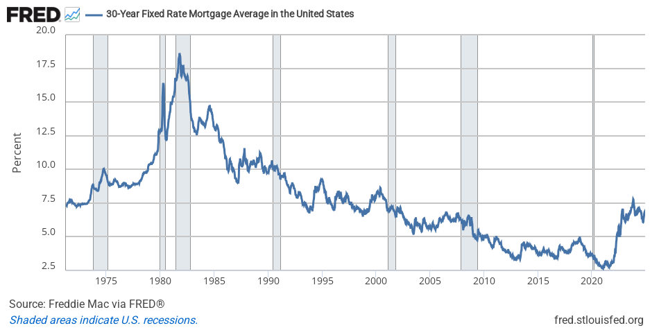
You’re buying a $500,000 house, putting $100,000 down, and borrowing $400,000 at a 7% annual rate (about right for 2024-2026 levels), 30 years, monthly payments. What’s the monthly payment?

Convert annual to monthly: $r_m = 0.07/12 = 0.005833$ per month; $T = 360$ months. Set PV of the annuity = $400,000 and solve for $C$:

$$400,\!000 = C \times \frac{1 - (1.005833)^{-360}}{0.005833}.$$

The annuity factor: $\frac{1 - 0.1232}{0.005833} = 150.31$.

$$C = \frac{400,\!000}{150.31} \approx \$2,\!661 \text{ per month}.$$

This is why the change from a 3% mortgage to a 7% mortgage in 2022-2023 was so painful for homebuyers. At 3%, the same $400,000 mortgage is about $1,686/month, a difference of $1,000/month for the same house. Lennar’s mortgage-rate buydowns (mentioned in the ECO 1002 IS-LM lesson) exist exactly to close part of that gap for new buyers.

A small reminder

These formulas all assume payments at the end of each period (ordinary annuity). If payments come at the start of each period (annuity due, like rent), multiply the PV by $(1 + r)$. The difference is one period of compounding.

Where this leads

Bond pricing in the next lesson is a coupon annuity plus a face-value lump sum. Stock valuation in Unit 3 is a growing perpetuity (or multi-stage version). Mortgages, leases, and pensions are all annuities. Master these four formulas and most fixed-income valuation reduces to plug-and-chug.